TikZ and PGF Manual
Graph Drawing
30 Graph Drawing Layouts: Trees
by Till Tantau
-
Graph Drawing Library trees 
\usegdlibrary{trees} %
LaTeX
and plain
TeX
\usegdlibrary[trees] % ConTeXt
TikZ offers several different syntax to specify trees (see Sections 19 and 21). The job of the graph drawing algorithms from this library is to turn the specification of trees into beautiful layouts.
We start this section with a description of algorithms, then we have a look at how missing children can be specified and at what happens when the input graph is not a tree.
30.1 The Tree Layouts
30.1.1 The Reingold–Tilford Layout
-
/graph drawing/tree layout=⟨string⟩ 
-
• E. M. Reingold and J. S. Tilford, Tidier drawings of trees, IEEE Transactions on Software Engineering, 7(2), 223–228, 1981.
-
• A. Brüggemann-Klein, D. Wood, Drawing trees nicely with TeX, Electronic Publishing, 2(2), 101–115, 1989.
-
1. For a node, recursively compute a layout for each of its children.
-
2. Place the tree rooted at the first child somewhere on the page.
-
3. Place the tree rooted at the second child to the right of the first one as near as possible so that no two nodes touch (and such that the sibling sep padding is not violated).
-
4. Repeat for all subsequent children.
-
5. Then place the root above the child trees at the middle position, that is, at the half-way point between the left-most and the right-most child of the node.
This layout uses the Reingold–Tilform method for drawing trees. The Reingold–Tilford method is a standard method for drawing trees. It is described in:
My implementation in graphdrawing.trees follows the following paper, which introduces some nice extensions of the basic algorithm:
As a historical remark, Brüggemann-Klein and Wood have implemented their version of the Reingold–Tilford algorithm directly in TeX (resulting in the TreeTeX style). With the power of LuaTeX at our disposal, the 2012 implementation in the graphdrawing.tree library is somewhat more powerful and cleaner, but it really was an impressive achievement to implement this algorithm back in 1989 directly in TeX.
The basic idea of the Reingold–Tilford algorithm is to use the following rules to position the nodes of a tree (the following description assumes that the tree grows downwards, other growth directions are handled by the automatic orientation mechanisms of the graph drawing library):
The standard keys level distance, level sep, sibling distance, and sibling sep, as well as the pre and post versions of these keys, as taken into consideration when nodes are positioned. See also Section 28.3 for details on these keys.
Handling of Missing Children. As described in Section 30.2, you can specify that some child nodes are “missing” in the tree, but some space should be reserved for them. This is exactly what happens: When the subtrees of the children of a node are arranged, each position with a missing child is treated as if a zero-width, zero-height subtree were present at that positions:
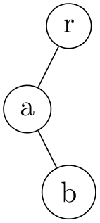
or in graph syntax:
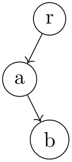
More than one child can go missing:
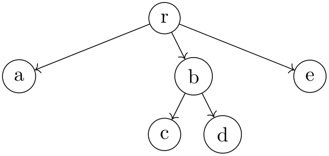
                    \usetikzlibrary {graphs,graphdrawing} \usegdlibrary {trees}

                    \tikz \graph [tree layout, nodes={draw,circle}, sibling sep=0pt]

                      { r
                    -> { a, , ,b
                    -> {c,d}, ,e} };
Although missing children are taken into consideration for the computation of the placement of the children of a root node relative to one another and also for the computation of the position of the root node, they are usually not considered as part of the “outline” of a subtree (the minimum number of children key ensures that b, c, e, and f all have a missing right child):
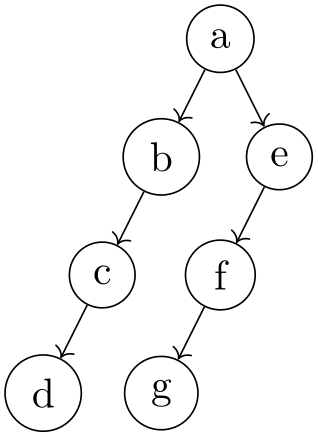
This behaviour of “ignoring” missing children in later stages of the recursion can be changed using the key missing nodes get space.
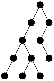
Significant Pairs of Siblings. Brüggemann-Klein and Wood have proposed an extension of the Reingold–Tilford method that is intended to better highlight the overall structure of a tree. Consider the following two trees:

                    \usetikzlibrary {graphs,graphdrawing} \usegdlibrary {trees}

                    \tikz [baseline=(a.base), tree layout, minimum number of children=2,

                           sibling distance=5mm, level distance=5mm]

                      \graph [nodes={circle, inner sep=0pt, minimum size=2mm, fill, as=}]{

                        a
                    -- { b
                    --
                    c
                    -- { d
                    --
                    e, f
                    -- { g, h }}, i
                    --
                    j
                    --
                    k[second] }

                      };\quad

                    \tikz [baseline=(a.base), tree layout, minimum number of children=2,

                           sibling distance=5mm, level distance=5mm]

                      \graph [nodes={circle, inner sep=0pt, minimum size=2mm, fill, as=}]{

                        a
                    -- { b
                    --
                    c
                    --
                    d
                    --
                    e, i
                    --
                    j
                    -- { f
                    -- {g,h}, k
                    } }

                      };
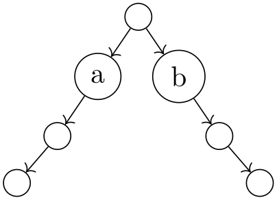
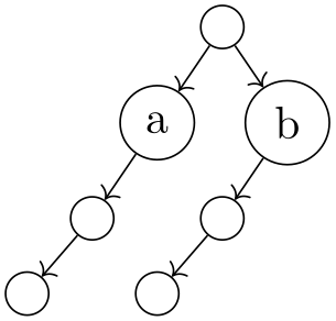
As observed by Brüggemann-Klein and Wood, the two trees are structurally quite different, but the Reingold–Tilford method places the nodes at exactly the same positions and only one edge “switches” positions. In order to better highlight the differences between the trees, they propose to add a little extra separation between siblings that form a significant pair. They define such a pair as follows: Consider the subtrees of two adjacent siblings. There will be one or more levels where these subtrees have a minimum distance. For instance, the following two trees the subtrees of the nodes a and b have a minimum distance only at the top level in the left example, and in all levels in the second example. A significant pair is a pair of siblings where the minimum distance is encountered on any level other than the first level. Thus, in the first example there is no significant pair, while in the second example a and b form such a pair.
                    \usetikzlibrary {graphs,graphdrawing} \usegdlibrary {trees}

                    \tikz \graph [tree layout, minimum number of children=2,

                                   level distance=5mm, nodes={circle,draw}]

                      { /
                    -> { a
                    ->
                    /
                    ->
                    /, b
                    ->
                    /[second] ->
                    /[second] }};

                      \quad

                    \tikz \graph [tree layout, minimum number of children=2,

                                  level distance=5mm, nodes={circle,draw}]

                      { /
                    -> { a
                    ->
                    /
                    ->
                    /, b
                    ->
                    /
                    ->
                    / }};
Whenever the algorithm encounters a significant pair, it adds extra space between the siblings as specified by the significant sep key.
Examples

-
/graph drawing/missing nodes get space=⟨boolean⟩(default true) 
When set to true, missing children are treated as if they where zero-width, zero-height nodes during the whole tree layout process.
Example
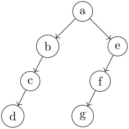
                    \tikz \graph [tree layout, missing nodes get space,

                                  minimum number of children=2, nodes={draw,circle}]

                    { a
                    -> { b
                    ->
                    c
                    ->
                    d, e
                    ->
                    f
                    ->
                    g } };
-
/graph drawing/significant sep=⟨length⟩(initially 0) 
This space is added to significant pairs by the modified Reingold–Tilford algorithm.
Example
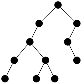

                    \tikz [baseline=(a.base), tree layout, significant sep=1em,

                           minimum number of children=2,

                           sibling distance=5mm, level distance=5mm]

                      \graph [nodes={circle, inner sep=0pt, minimum size=2mm, fill, as=}]{

                        a
                    -- { b
                    --
                    c
                    -- { d
                    --
                    e, f
                    -- { g, h }}, i
                    --
                    j
                    --
                    k[second] }

                      };\quad

                    \tikz [baseline=(a.base), tree layout, significant sep=1em,

                           minimum number of children=2,

                           sibling distance=5mm, level distance=5mm]

                      \graph [nodes={circle, inner sep=0pt, minimum size=2mm, fill, as=}]{

                        a
                    -- { b
                    --
                    c
                    --
                    d
                    --
                    e, i
                    --
                    j
                    -- { f
                    -- {g,h}, k
                    } }

                      };
-
/graph drawing/binary tree layout=⟨string⟩ 
-
1. tree layout, thereby selecting the Reingold–Tilford method,
-
2. minimum number of children=2, thereby ensuring the all nodes have (at least) two children or none at all, and
-
3. significant sep=10pt to highlight significant pairs.
A layout based on the Reingold–Tilford method for drawing binary trees. This key executes:
In the examples, the last one is taken from the paper of Brüggemann-Klein and Wood. It demonstrates nicely the advantages of having the full power of TikZ’s anchoring and the graph drawing engine’s orientation mechanisms at one’s disposal.
Examples

                    \tikz [grow'=up, binary tree layout, sibling distance=7mm, level distance=7mm]

                      \graph {

                        a
                    -- { b
                    --
                    c
                    -- { d
                    --
                    e, f
                    -- { g, h }}, i
                    --
                    j
                    --
                    k[second] }

                      };
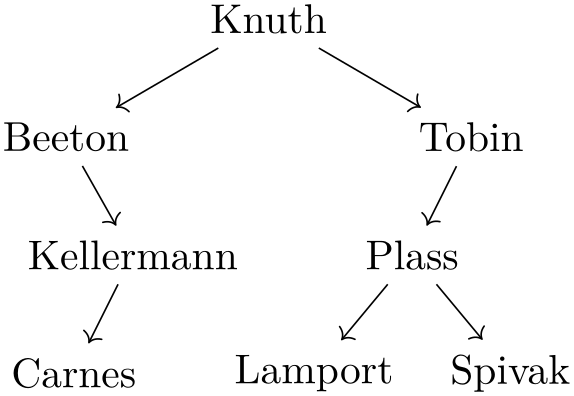
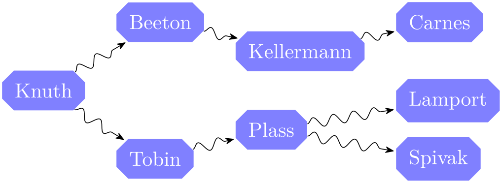
                    \tikz \graph [binary tree layout] {

                      Knuth
                    -> {

                        Beeton
                    ->
                    Kellermann [second] ->
                    Carnes,

                        Tobin
                    ->
                    Plass
                    -> { Lamport, Spivak }

                      }

                    };\qquad

                    \tikz [>={Stealth[round,sep]}]

                      \graph [binary tree layout, grow'=right, level sep=1.5em,

                              nodes={right, fill=blue!50, text=white, chamfered
                      rectangle},

                                     edges={decorate,decoration={snake, post
                      length=5pt}}]

                      {

                        Knuth
                    -> {

                          Beeton
                    ->
                    Kellermann [second] ->
                    Carnes,

                          Tobin
                    ->
                    Plass
                    -> { Lamport, Spivak }

                        }

                      };
-
/graph drawing/extended binary tree layout=⟨string⟩ 
This algorithm is similar to binary tree layout, only the option missing nodes get space is executed and the significant sep is zero.
Example
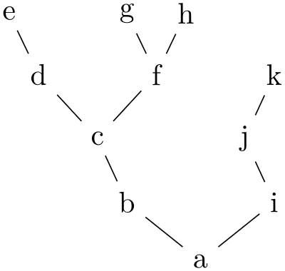
                    \tikz [grow'=up, extended binary tree layout,

                           sibling distance=7mm, level distance=7mm]

                      \graph {

                        a
                    -- { b
                    --
                    c
                    -- { d
                    --
                    e, f
                    -- { g, h }}, i
                    --
                    j
                    --
                    k[second] }

                      };
30.2 Specifying Missing Children
In the present section we discuss keys for specifying missing children in a tree. For many certain kind of trees, in particular for binary trees, there are not just “a certain number of children” at each node, but, rather, there is a designated “first” (or “left”) child and a “second” (or “right”) child. Even if one of these children is missing and a node actually has only one child, the single child will still be a “first” or “second” child and this information should be taken into consideration when drawing a tree.
The first useful key for specifying missing children is missing number of children which allows you to state how many children there are, at minimum.
Once the minimum number of children has been set, we still need a way of specifying “missing first children” or, more generally, missing children that are not “at the end” of the list of children. For this, there are three methods:
-
1. When you use the child syntax, you can use the missing key with the child command to indicate a missing child:
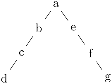
-
2. When using the graph syntax, you can use an “empty node”, which really must be completely empty and may not even contain a slash, to indicate a missing node:

                    \usetikzlibrary {graphs,graphdrawing} \usegdlibrary {trees}

                     \tikz [binary tree layout, level distance=5mm]

                     \graph { a
                    -> { b
                    ->
                    c
                    ->
                    d, e
                    -> { , f
                    -> { , g} } } };
-
3. You can simply specify the index of a child directly using the key desired child index.
-
/graph drawing/minimum number of children=⟨number⟩(initially 0) 
Specifies how many children a tree node must have at least. If there are less, “virtual” children are added. When this key is set to 2 or more, the following happens: We first compute a spanning tree for the graph, see Section 30.3. Then, whenever a node is not a leaf in this spanning tree (when it has at least one child), we add “virtual” or “dummy” nodes as children of the node until the total number of real and dummy children is at least ⟨number⟩. If there where at least ⟨number⟩ children at the beginning, nothing happens.
The new children are added after the existing children. This means that, for instance, in a tree with ⟨number⟩ set to 2, for every node with a single child, this child will be the first child and the second child will be missing.
Example
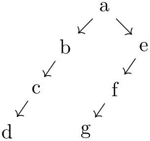
                    \tikz \graph [binary tree layout,level distance=5mm]

                    { a
                    -> { b->c->d, e->f->g } };
-
/graph drawing/desired child index=⟨number⟩ 
Pass this key to a node to tell the graph drawing engine which child number you “desired” for the node. Whenever all desires for the children of a node are conflict-free, they will all be met; children for which no desired indices were given will remain at their position, whenever possible, but will “make way” for children with a desired position. In detail, the following happens: We first determine the total number of children (real or dummy) needed, which is the maximum of the actual number of children, of the minimum number of children, and of the highest desired child index. Then we go over all children that have a desired child index and put they at this position. If the position is already taken (because some other child had the same desired index), the next free position is used with a wrap-around occurring at the end. Next, all children without a desired index are place using the same mechanism, but they want to be placed at the position they had in the original spanning tree.
While all of this might sound a bit complicated, the application of the key in a binary tree is pretty straightforward: To indicate that a node is a “right” child in a tree, just add desired child index=2 to it. This will make it a second child, possibly causing the first child to be missing. If there are two nodes specified as children of a node, by saying desired child index=⟨number⟩ for one of them, you will cause it be first or second child, depending on ⟨number⟩, and cause the other child to become the other child.
Since desired child index=2 is a bit long, the following shortcuts are available: first, second, third, and fourth. You might wonder why second is used rather than right. The reason is that trees may also grow left and right and, additionally, the right and left keys are already in use for anchoring. Naturally, you can locally redefine them, if you want.
Examples

                    \tikz \graph [binary tree layout, level distance=5mm]

                    { a
                    ->
                    b[second] };
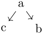
                    \tikz \graph [binary tree layout, level distance=5mm]

                    { a
                    -> { b[second], c} };
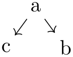
                    \tikz \graph [binary tree layout, level distance=5mm]

                    { a
                    -> { b, c[first]} };
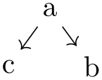
                    \tikz \graph [binary tree layout, level distance=5mm]

                    { a
                    -> { b[second], c[second]} };
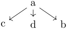
                    \tikz \graph [binary tree layout, level distance=5mm]

                    { a
                    -> { b[third], c[first], d} };
-
/graph drawing/first=⟨string⟩ 
A shorthand for setting the desired child number to 1.
-
/graph drawing/second=⟨string⟩ 
A shorthand for setting the desired child number to 2.
-
/graph drawing/third=⟨string⟩ 
A shorthand for setting the desired child number to 3.
-
/graph drawing/fourth=⟨string⟩ 
A shorthand for setting the desired child number to 4.
30.3 Spanning Tree Computation
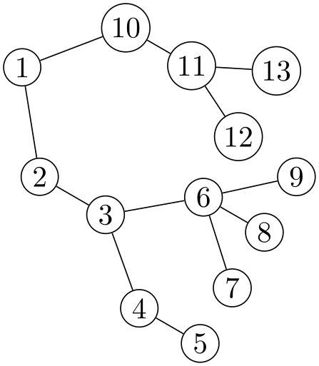
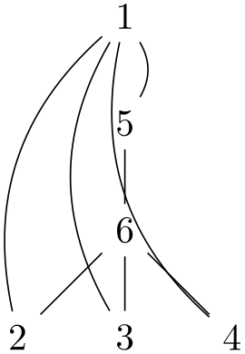
Although the algorithms of this library are tailored to layout trees, they will work for any graph as input. First, if the graph is not connected, it is decomposed into connected components and these are laid out individually. Second, for each component, a spanning tree of the graph is computed first and the layout is computed for this spanning tree; all other edges will still be drawn, but they have no impact on the placement of the nodes. If the graph is already a tree, the spanning tree will be the original graph.
The computation of the spanning tree is a non-trivial process since a non-tree graph has many different possible spanning trees. You can choose between different methods for deciding on a spanning tree, it is even possible to implement new algorithms. (In the future, the computation of spanning trees and the cycle removal in layered graph drawing algorithms will be unified, but, currently, they are implemented differently.)
Selects the (sub)algorithm that is to be used for computing spanning trees whenever this is requested by a tree layout algorithm. The default algorithm is breadth first spanning tree.
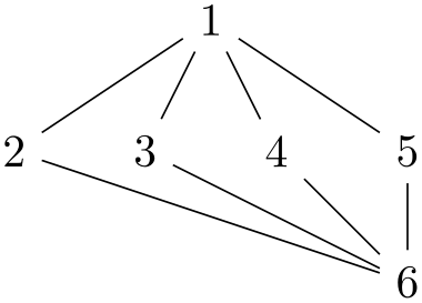
                \usetikzlibrary {graphs,graphdrawing} \usegdlibrary {trees}

                \tikz \graph [tree layout, breadth first spanning tree]

                {

                  1
                -- {2,3,4,5} --
                6;

                };
                \usetikzlibrary {graphs,graphdrawing} \usegdlibrary {trees}

                \tikz \graph [tree layout, depth first spanning tree]

                {

                  1
                --[bend right] {2,3,4,5 [>bend left]} --
                6;

                };
-
/graph drawing/breadth first spanning tree=⟨string⟩ 
-
1. It looks for a node for which the root parameter is set. If there are several such nodes, the first one is used. If there are no such nodes, the first node is used.
Let call the node determined in this way the root node.
-
2. For every edge, a priority is determined, which is a number between 1 and 10. How this happens, exactly, will be explained in a moment. Priority 1 means “most important” while priority 10 means “least important”.
-
3. Starting from the root node, we now perform a breadth first search through the tree, thereby implicitly building a spanning tree: Suppose for a moment that all edges have priority 1. Then, the algorithm works just the way that a normal breadth first search is performed: We keep a queue of to-be-visited nodes and while this queue is not empty, we remove its first node. If this node has not yet been visited, we add all its neighbors at the end of the queue. When a node is taken out of the queue, we make it the child of the node whose neighbor it was when it was added. Since the queue follows the “first in, first out” principle (it is a fifo queue), the children of the root will be all nodes at distance \(1\) form the root, their children will be all nodes at distance \(2\), and so on.
-
4. Now suppose that some edges have a priority different from 1, in which case things get more complicated. We now keep track of one fifo queue for each of the ten possible priorities. When we consider the neighbors of a node, we actually consider all its incident edges. Each of these edges has a certain priority and the neighbor is put into the queue of the edge’s priority. Now, we still remove nodes normally from the queue for priority 1; only if this queue is empty and there is still a node in the queue for priority 2 we remove the first element from this queue (and proceed as before). If the second queue is also empty, we try the third, and so on up to the tenth queue. If all queues are empty, the algorithm stops.
This key selects “breadth first” as the (sub)algorithm for computing spanning trees. Note that this key does not cause a graph drawing scope to start; the key only has an effect in conjunction with keys like tree layout. The algorithm will be called whenever a graph drawing algorithm needs a spanning tree on which to operate. It works as follows:
The effect of the ten queues is the following: If the edges of priority \(1\) span the whole graph, a spanning tree consisting solely of these edges will be computed. However, if they do not, once we have visited reachable using only priority 1 edges, we will extend the spanning tree using a priority 2 edge; but then we once switch back to using only priority 1 edges. If neither priority 1 nor priority 2 edges suffice to cover the whole graph, priority 3 edges are used, and so on.
-
/graph drawing/depth first spanning tree=⟨string⟩ 
Works exactly like breadth first spanning tree (same handling of priorities), only the queues are now lifo instead of fifo.
-
/graph drawing/root=⟨boolean⟩(default true) 
This Boolean parameter is used in the computation of spanning trees. When can be set for a node, this node will be used as the root for the spanning tree computation. If several nodes have this option set, the first node will be used.
-
/graph drawing/span priority=⟨number⟩ 
Explicitly sets the “span priority” of an edge to ⟨number⟩, which must be a number between 1 and 10. The priority of edges is used by spanning tree computations, see breadth first spanning tree.
-
/graph drawing/span edge=⟨string⟩ 
An easy-to-remember shorthand for span priority=1. When this key is used with an edge, it will always be preferred over other edges
-
/graph drawing/no span edge=⟨string⟩ 
An easy-to-remember shorthand for span priority=10. This causes the edge to be used only as a last resort as part of a spanning tree. In the example, we add lots of edges that would normally be preferred in the computation of the spanning tree, but use no span edge to cause the algorithm to ignore these edges.
Example

                    \tikz \graph [tree layout, nodes={draw}, sibling distance=0pt,

                                  every group/.style={

                                    default edge kind=->, no span edge,

                                    path=source}]

                    {

                      5
                    -> {

                        "1,3"
                    -> {0,2,4},

                        11    ->
                    {

                          "7,9"
                    -> { 6, 8, 10
                    }

                        }

                      }

                    };
-
/graph drawing/span priority ->=⟨number⟩(initially 3) 
-
• span priority -> = 3
-
• span priority -- = 5
-
• span priority <-> = 5
-
• span priority <- = 8
-
• span priority -!- = 10
This key stores the span priority of all edges whose direction is ->. There are similar keys for all other directions, such as span priority <- and so on. When you write
                    graph { a
                    ->
                    b
                    --
                    c
                    <- [span priority=2] d
                    }
the priority of the edge from a to b would be the current value of the key span priority ->, the priority of the edge from b to c would be the current value of span priority --, and the priority of the edge from c to d would be 2, regardless of the value of span priority <-.
The defaults for the priorities are:
-
/graph drawing/span priority reversed ->=⟨number⟩(initially 9) 
-
• span priority reversed -> = 9
-
• span priority reversed -- = 5
-
• span priority reversed <-> = 5
-
• span priority reversed <- = 7
-
• span priority reversed -!- = 10
When you write
                    graph { a
                    ->
                    b
                    --
                    c
                    <- [span priority=2] d
                    }
there are, in addition to the priorities indicated above, also further edge priorities: The priority of the (reversed) edge b to a is span priority reversed ->, the priority of the (reversed) edge c to b is span priority reversed --, and the span priority of the reversed edge d to c is 2, regardless of the value of span priority reversed <-.
The defaults for the priorities are:
The default priorities are set in such a way, that non-reversed -> edges have top priorities, -- and <-> edges have the same priorities in either direction, and <- edges have low priority in either direction (but going a <- b from b to a is given higher priority than going from a to b via this edge and also higher priority than going from b to a in a -> b).
Keys like span using directed change the priorities “en bloc”.
-
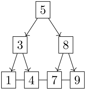
/graph drawing/span using directed=⟨string⟩ 
This style sets a priority of 3 for all edges that are directed and “go along the arrow direction”, that is, we go from a to b with a priority of 3 for the cases a -> b, b <- a, a <-> b, and b <-> a. This strategy is nice with trees specified with both forward and backward edges.
Example
-
/graph drawing/span using all=⟨string⟩ 
Assigns a uniform priority of 5 to all edges.