TikZ and PGF Manual
Graph Drawing
28 Using Graph Drawing in TikZ
by Till Tantau
-
TikZ Library graphdrawing 
\usetikzlibrary{graphdrawing} %
LaTeX
and plain
TeX
\usetikzlibrary[graphdrawing] % ConTeXt
This package provides capabilities for automatic graph drawing. It requires that the document is typeset using LuaTeX. This package should work with LuaTeX
0.54 or higher.
28.1 Choosing a Layout and a Library
The graph drawing engine is initialized when you load the library graphdrawing. This library provides the basic framework for graph drawing, including all options and keys described in the present section. However, this library does not load any actual algorithms for drawing graphs. For this, you need to use the following command, which is defined by the graphdrawing library:
-
\usegdlibrary{⟨list of libraries⟩} 
-
1. Check whether LuaTeX can call require on the library file pgf.gd.⟨name⟩.library. LuaTeX’s usual file search mechanism will search the texmf-trees in the usual manner and the dots in the file name get converted into directory slashes.
-
2. If the above failed, try to require the string pgf.gd.⟨name⟩.
-
3. If this fails, try to require the string ⟨name⟩.library.
-
4. If this fails, try to require the string ⟨name⟩. If this fails, print an error message.
This command is used to load the special graph drawing libraries (the gd in the name of the command stands for “graph drawing”). The ⟨list of libraries⟩ is a comma-separated list of library written in the Lua programming language (which is why a special command is needed).
In detail, this command does the following. For each ⟨name⟩ in the ⟨list of libraries⟩ we do:
The net effect of the above is the following: Authors of graph drawing algorithms can bundle together multiple algorithms in a library by creating a ...xyz/library.lua file that internally just calls require for all files containing declarations. On the other hand, if a graph drawing algorithm completely fits inside a single file, it can also be read directly using \usegdlibrary.
The different graph drawing libraries are documented in the following Sections 30 to 35.
Note that in addition to the graph drawing libraries, you may also wish to load the normal TikZ library graphs. It provides the powerful graph path command with its easy-to-use syntax for specifying graphs, but you can use the graph drawing engine independently of the graphs library, for instance in conjunction with the child or the edge syntax. Here is a typical setup:
                \usetikzlibrary{graphs, graphdrawing}

                \usegdlibrary{trees, layered}
Having set things up, you must then specify for which scopes the graph drawing engine should apply a layout algorithm to the nodes in the scope. Typically, you just add an option ending with ... layout to the graph path operation and then let the graph drawing do its magic:
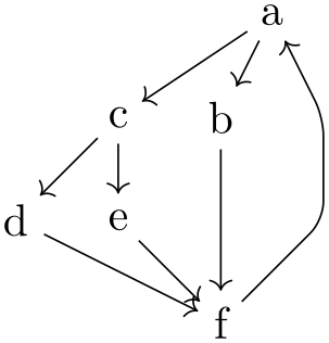
                \usetikzlibrary {graphs,graphdrawing} \usegdlibrary {layered}

                \tikz [rounded corners]

                  \graph [layered layout, sibling distance=8mm, level distance=8mm]

                  {

                    a
                -> {

                      b,

                      c
                -> { d, e }

                    } ->

                    f
                ->

                    a

                  };
Whenever you use such an option, you can:
-
• Create nodes in the usual way. The nodes will be created completely, but then tucked away in an internal table. This means that all of TikZ’s options for nodes can be applied. You can also name a node and reference it later.
-
• Create edges using either the syntax of the graph command (using --, <-, ->, or <->), or using the edge command, or using the child command. These edges will, however, not be created immediately. Instead, the basic layer’s command \pgfgdedge will be called, which stores “all the information concerning the edge”. The actual drawing of the edge will only happen after all nodes have been positioned.
-
• Most of the keys that can be passed to an edge will work as expected. In particular, you can add labels to edges using the usual node syntax for edges.
-
• The label and pin options can be used in the usual manner with nodes inside a graph drawing scope. Only, the labels and nodes will play no role in the positioning of the nodes and they are added when the nodes are finally positioned.
-
• Similarly, nodes that are placed “on an edge” using the implicit positioning syntax can be used in the usual manner.
Here are some things that will not work:
-
• Only edges created using the graph syntax, the edge command, or the child command will correctly pass their connection information to the basic layer. When you write \draw (a)--(b); inside a graph drawing scope, where a and b are nodes that have been created inside the scope, you will get an error message / things will look wrong. The reason is that the usual -- is not “caught” by the graph drawing engine and, thus, tries to immediately connect two nodes that do not yet exist (except inside some internal table).
-
• The options of edges are executed twice: Once when the edge is “examined” by the \pgfgdedge command (using some magic to shield against the side effects) and then once more when the edge is actually created. Fortunately, in almost all cases, this will not be a problem; but if you do very evil magic inside your edge options, you must roll a D100 to see what strange things will happen. (Do no evil, by the way.)
If you are really interested in the “fine print” of what happens, please see Section 29.
28.2 Graph Drawing Parameters
Graph drawing algorithms can typically be configured in some way. For instance, for a graph drawing algorithm that visualizes its nodes as a tree, it will typically be useful when the user can change the so-called level distance and the sibling distance. For other algorithms, like force-based algorithms, a large number of parameters influence the way the algorithms work. Options that influence graph drawing algorithms will be called (graph drawing) parameters in the following. From the user’s point of view, these parameters look like normal TikZ keys and you set them in the usual way. Internally, they are treated a bit differently from normal keys since their “effect” becomes apparent only later on, namely during the run of the graph drawing algorithm.
A graph drawing algorithm may or may not take different graph parameters into account. After all, these options may even outright contradict each other, so an algorithm can only try to “do its best”. While many graph parameters are very specific to a single algorithm, a number of graph parameters will be important for many algorithms and they are documented in the course of the present section. Here is an example of an option the “always works”:
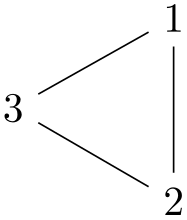
                \usetikzlibrary {graphs,graphdrawing} \usegdlibrary {force}

                \tikz \graph [spring layout, vertical=1 to 2] { 1--2--3--1
                };
28.3 Padding and Node Distances
In many drawings, you may wish to specify how “near” two nodes should be placed by a graph drawing algorithm. Naturally, this depends strongly on the specifics of the algorithm, but there are a number of general keys that will be used by many algorithms.
There are different kinds of objects for which you can specify distances and paddings:
-
• You specify the “natural” distance between nodes connected by an edge using node distance, which is also available in normal TikZ albeit for a slightly different purpose. However, not every algorithm will (or can) honor the key; see the description of each algorithm what it will “make of this option”.
-
• A number of graph drawing algorithms arrange nodes in layers (or levels); we refer to the nodes on the same layer as siblings (although, in a tree, siblings are only nodes with the same parent; nevertheless we use “sibling” loosely also for nodes that are more like “cousins”).
-
• When a graph consists of several connected component, many graph drawing algorithms will layout these components individually. The different components will then be arranged next to each other, see Section 28.7 for the details, such that between the nodes of any two components a padding is available.
-
/graph drawing/node distance=⟨length⟩(initially 1cm)
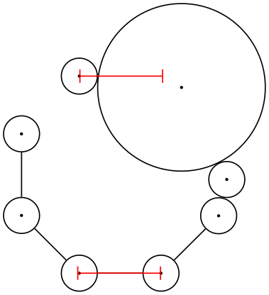
This is minimum distance that the centers of nodes connected by an edge should have. It will not always be possible to satisfy this desired distance, for instance in case the nodes are too big. In this case, the ⟨length⟩ is just considered as a lower bound.
Example
                    \begin{tikzpicture}

                      \graph [simple necklace layout,  node distance=1cm, node sep=0pt,

                              nodes={draw,circle,as=.}]

                      {

                        1
                    --
                    2 [minimum size=2cm] --
                    3
                    --

                        4
                    --
                    5
                    --
                    6
                    --
                    7
                    --[orient=up] 8

                      };

                      \draw [red,|-|] (1.center) --
                    ++(0:1cm);

                      \draw [red,|-|] (5.center) --
                    ++(180:1cm);

                    \end{tikzpicture}
-
/graph drawing/node pre sep=⟨length⟩(initially .333em) 
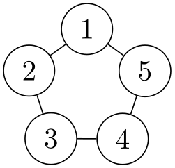
This is a minimum “padding” or “separation” between the border of nodes connected by an edge. Thus, if nodes are so big that nodes with a distance of node distance would overlap (or just come with ⟨dimension⟩ distance of one another), their distance is enlarged so that this distance is still satisfied. The pre means that the padding is added to the node “at the front”. This make sense only for some algorithms, like for a simple necklace layout.
Examples
                    \tikz \graph [simple necklace layout, node distance=0cm, nodes={circle,draw}]

                      { 1--2--3--4--5--1 };

                    \tikz \graph [simple necklace layout, node distance=0cm, node sep=0mm,

                                  nodes={circle,draw}]

                      { 1--2--3[node pre sep=5mm]--4--5[node pre sep=1mm]--1
                    };
-
/graph drawing/node post sep=⟨length⟩(initially .333em) 
Works like node pre sep.
-
/graph drawing/node sep=⟨length⟩ 
A shorthand for setting both node pre sep and node post sep to \(\meta {length}/2\).
-
/graph drawing/level distance=⟨length⟩(initially 1cm)
This is minimum distance that the centers of nodes on one level should have from the centers of nodes on the next level. It will not always be possible to satisfy this desired distance, for instance in case the nodes are too big. In this case, the ⟨length⟩ is just considered as a lower bound.
Example

                    \begin{tikzpicture}[inner sep=2pt]

                      \draw [help lines] (0,0) grid
                    (3.5,2);

                      \graph [layered layout, level distance=1cm, level sep=0]

                        { 1 [x=1,y=2] --
                    2
                    --
                    3
                    --
                    1 };

                      \graph [layered layout, level distance=5mm, level sep=0]

                        { 1 [x=3,y=2] --
                    2
                    --
                    3
                    --
                    1, 3
                    -- {4,5} --
                    6
                    --
                    3 };

                    \end{tikzpicture}
-
/graph drawing/layer distance=⟨length⟩ 
An alias for level distance
-
/graph drawing/level pre sep=⟨length⟩(initially .333em) 
This is a minimum “padding” or “separation” between the border of the nodes on a level to any nodes on the previous level. Thus, if nodes are so big that nodes on consecutive levels would overlap (or just come with ⟨length⟩ distance of one another), their distance is enlarged so that this distance is still satisfied. If a node on the previous level also has a level post sep, this post padding and the ⟨dimension⟩ add up. Thus, these keys behave like the “padding” keys rather than the “margin” key of cascading style sheets.
Example
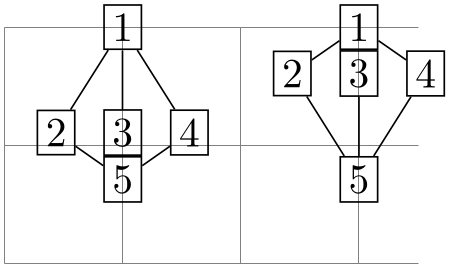
                    \begin{tikzpicture}[inner sep=2pt, level sep=0pt, sibling distance=0pt]

                      \draw [help lines] (0,0) grid
                    (3.5,2);

                      \graph [layered layout, level distance=0cm, nodes=draw]

                        { 1 [x=1,y=2] --
                    {2,3[level pre sep=1mm],4[level pre sep=5mm]} --
                    5 };

                      \graph [layered layout, level distance=0cm, nodes=draw]

                        { 1 [x=3,y=2] --
                    {2,3,4} --
                    5[level pre sep=5mm] };

                    \end{tikzpicture}
-
/graph drawing/level post sep=⟨length⟩(initially .333em) 
Works like level pre sep.
-
/graph drawing/layer pre sep=⟨length⟩ 
An alias for level pre sep.
-
/graph drawing/layer post sep=⟨length⟩ 
An alias for level post sep.
-
/graph drawing/level sep=⟨length⟩ 
A shorthand for setting both level pre sep and level post sep to \(\meta {length}/2\). Note that if you set level distance=0 and level sep=1em, you get a layout where any two consecutive layers are “spaced apart” by 1em.
-
/graph drawing/layer sep=⟨number⟩ 
An alias for level sep.
-
/graph drawing/sibling distance=⟨length⟩(initially 1cm)
This is minimum distance that the centers of node should have to the center of the next node on the same level. As for levels, this is just a lower bound. For some layouts, like a simple necklace layout, the ⟨length⟩ is measured as the distance on the circle.
Examples
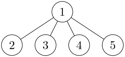
                    \tikz \graph [tree layout, sibling distance=1cm, nodes={circle,draw}]

                      { 1--{2,3,4,5} };
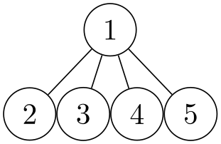
                    \tikz \graph [tree layout, sibling distance=0cm, sibling sep=0pt,

                                  nodes={circle,draw}]

                      { 1--{2,3,4,5} };

                    \tikz \graph [tree layout, sibling distance=0cm, sibling sep=0pt,

                                  nodes={circle,draw}]

                      { 1--{2,3[sibling distance=1cm],4,5} };
-
/graph drawing/sibling pre sep=⟨length⟩(initially .333em) 
Works like level pre sep, only for siblings.
Example
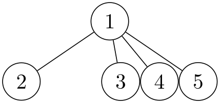
                    \tikz \graph [tree layout, sibling distance=0cm, nodes={circle,draw},

                                  sibling sep=0pt]

                      { 1--{2,3[sibling pre sep=1cm],4,5} };
-
/graph drawing/sibling post sep=⟨length⟩(initially .333em) 
Works like sibling pre sep.
-
/graph drawing/sibling sep=⟨length⟩ 
A shorthand for setting both sibling pre sep and sibling post sep to \(\meta {length}/2\).
-
/graph drawing/part distance=⟨length⟩(initially 1.5cm) 
This is minimum distance between the centers of “parts” of a graph. What a “part” is depends on the algorithm.
-
/graph drawing/part pre sep=⟨length⟩(initially 1em) 
A pre-padding for parts.
-
/graph drawing/part post sep=⟨length⟩(initially 1em) 
A post-padding for pars.
-
/graph drawing/part sep=⟨length⟩ 
A shorthand for setting both part pre sep and part post sep to \(\meta {length}/2\).
-
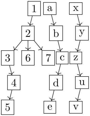
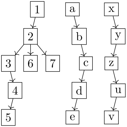
/graph drawing/component sep=⟨length⟩(initially 1.5em) 
This is padding between the bounding boxes that nodes of different connected components will have when they are placed next to each other.
Examples
-
/graph drawing/component distance=⟨length⟩(initially 2cm) 
This is the minimum distance between the centers of bounding boxes of connected components when they are placed next to each other. (Not used, currently.)
28.4 Anchoring a Graph
A graph drawing algorithm must compute positions of the nodes of a graph, but the computed positions are only relative (“this node is left of this node, but above that other node”). It is not immediately obvious where the “the whole graph” should be placed absolutely once all relative positions have been computed. In case that the graph consists of several unconnected components, the situation is even more complicated.
The order in which the algorithm layer determines the node at which the graph should be anchored:
-
1. If the anchor node=⟨node name⟩ option given to the graph as a whole, the graph is anchored at ⟨node name⟩, provided there is a node of this name in the graph. (If there is no node of this name or if it is misspelled, the effect is the same as if this option had not been given at all.)
-
2. Otherwise, if there is a node where the anchor here option is specified, the first node with this option set is used.
-
3. Otherwise, if there is a node where the desired at option is set (perhaps implicitly through keys like x), the first such node is used.
-
4. Finally, in all other cases, the first node is used.
In the above description, the “first” node refers to the node first encountered in the specification of the graph.
Once the node has been determined, the graph is shifted so that this node lies at the position specified by anchor at.
-
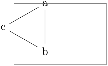
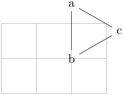
/graph drawing/desired at=⟨coordinate⟩ 
When you add this key to a node in a graph, you “desire” that the node should be placed at the ⟨coordinate⟩ by the graph drawing algorithm. Now, when you set this key for a single node of a graph, then, by shifting the graph around, this “wish” can obviously always be fulfill:
                    \usetikzlibrary {graphs,graphdrawing} \usegdlibrary {force}

                    \begin{tikzpicture}

                      \draw [help lines] (0,0) grid
                    (3,2);

                      \graph [spring layout]

                      {

                        a [desired at={(1,2)}] --
                    b
                    --
                    c
                    --
                    a;

                      };

                    \end{tikzpicture}
                    \usetikzlibrary {graphs,graphdrawing} \usegdlibrary {force}

                    \begin{tikzpicture}

                      \draw [help lines] (0,0) grid
                    (3,2);

                      \graph [spring layout]

                      {

                        a
                    --
                    b[desired at={(2,1)}] --
                    c
                    --
                    a;

                      };

                    \end{tikzpicture}
Since the key’s name is a bit long and since the many braces and parentheses are a bit cumbersome, there is a special support for this key inside a graph: The standard /tikz/at key is redefined inside a graph so that it points to /graph drawing/desired at instead. (Which is more logical anyway, since it makes no sense to specify an at position for a node whose position it to be computed by a graph drawing algorithm.) A nice side effect of this is that you can use the x and y keys (see Section 19.9.1) to specify desired positions:
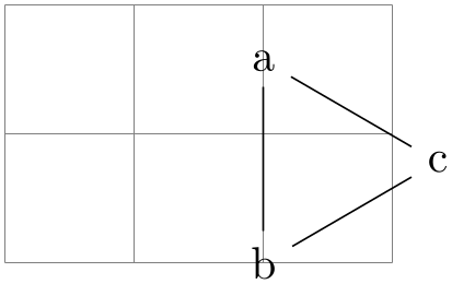
                    \usetikzlibrary {graphs,graphdrawing} \usegdlibrary {force}

                    \begin{tikzpicture}

                      \draw [help lines] (0,0) grid
                    (3,2);

                      \graph [spring layout]

                      {

                        a
                    --
                    b[x=2,y=0] --
                    c
                    --
                    a;

                      };

                    \end{tikzpicture}
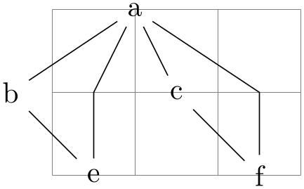
                    \usetikzlibrary {graphs,graphdrawing} \usegdlibrary {layered}

                    \begin{tikzpicture}

                      \draw [help lines] (0,0) grid
                    (3,2);

                      \graph [layered layout]

                      {

                        a [x=1,y=2] --
                    { b, c
                    } -- {e, f} --
                    a

                      };

                    \end{tikzpicture}
A problem arises when two or more nodes have this key set, because then your “desires” for placement and the positions computed by the graph drawing algorithm may clash. Graph drawing algorithms are “told” about the desired positions. Most algorithms will simply ignore these desired positions since they will be taken care of in the so-called post-anchoring phase, see below. However, for some algorithms it makes a lot of sense to fix the positions of some nodes and only compute the positions of the other nodes relative to these nodes. For instance, for a spring layout it makes perfect sense that some nodes are “nailed to the canvas” while other nodes can “move freely”.
Examples
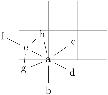
                    \begin{tikzpicture}

                      \draw [help lines] (0,0) grid
                    (3,2);

                      \graph [spring layout]

                      {

                        a[x=1] --
                    { b, c, d, e
                    -- {f,g,h} };

                        { h, g
                    } --
                    a;

                      };

                    \end{tikzpicture}

                    \begin{tikzpicture}

                      \draw [help lines] (0,0) grid
                    (3,2);

                      \graph [spring layout]

                      {

                        a
                    -- { b, c, d[x=0], e
                    -- {f[x=2], g, h[x=1]} };

                        { h, g
                    } --
                    a;

                      };

                    \end{tikzpicture}
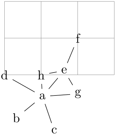
                    \begin{tikzpicture}

                      \draw [help lines] (0,0) grid
                    (3,2);

                      \graph [spring layout]

                      {

                        a
                    -- { b, c, d[x=0], e
                    -- {f[x=2,y=1], g, h[x=1]} };

                        { h, g
                    } --
                    a;

                      };

                    \end{tikzpicture}
-
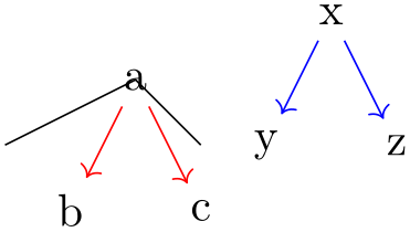
/graph drawing/anchor node=⟨string⟩ 
-
• at the current value of anchor at or
-
• at the position that is specified in the form of a desired at for the ⟨node name⟩.
This option can be used with a graph to specify a node that should be used for anchoring the whole graph. When this option is specified, after the layout has been computed, the whole graph will be shifted in such a way that the ⟨node name⟩ is either
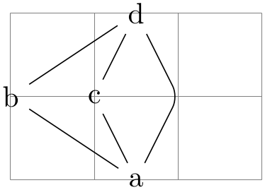
Note how in the last example c is placed at (1,1) rather than b as would happen by default.
Examples
                    \tikz \draw (0,0)

                      --
                    (1,0.5) graph
                    [edges=red,  layered layout, anchor node=a] { a
                    -> {b,c} }

                      --
                    (1.5,0) graph
                    [edges=blue, layered layout,

                                        anchor node=y, anchor at={(2,0)}]          { x
                    -> {y,z} };
                    \begin{tikzpicture}

                      \draw [help lines] (0,0) grid
                    (3,2);


                      \graph [layered layout, anchor node=c, edges=rounded corners]

                        { a
                    -- {b
                    [x=1,y=1], c
                    [x=1,y=1] } --
                    d
                    --
                    a};

                    \end{tikzpicture}
-
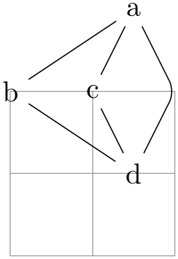
/graph drawing/anchor at=⟨canvas coordinate⟩(initially (0pt,0pt)) 
The coordinate at which the graph should be anchored when no explicit anchor is given for any node. The initial value is the origin.
Example
                    \begin{tikzpicture}

                      \draw [help lines] (0,0) grid
                    (2,2);


                      \graph [layered layout, edges=rounded corners, anchor at={(1,2)}]

                        { a
                    -- {b, c [anchor here] } --
                    d
                    --
                    a};

                    \end{tikzpicture}
-
/graph drawing/anchor here=⟨boolean⟩(default true) 
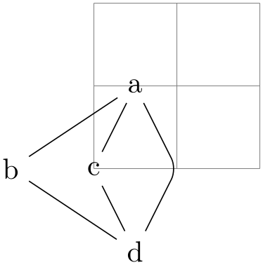
This option can be passed to a single node (rather than the graph as a whole) in order to specify that this node should be used for the anchoring process. In the example, c is placed at the origin since this is the default anchor at position.
Example
                    \begin{tikzpicture}

                      \draw [help lines] (0,0) grid
                    (2,2);


                      \graph [layered layout, edges=rounded corners]

                        { a
                    -- {b, c [anchor here] } --
                    d
                    --
                    a};

                    \end{tikzpicture}
28.5 Orienting a Graph
Just as a graph drawing algorithm cannot know where a graph should be placed on a page, it is also often unclear which orientation it should have. Some graphs, like trees, have a natural direction in which they “grow”, but for an “arbitrary” graph the “natural orientation” is, well, arbitrary.
There are two ways in which you can specify an orientation: First, you can specify that the line from a certain vertex to another vertex should have a certain slope. How these vertices and slopes are specified in explained momentarily. Second, you can specify a so-called “growth direction” for trees.
-
/graph drawing/orient=⟨direction⟩(default 0) 
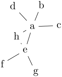
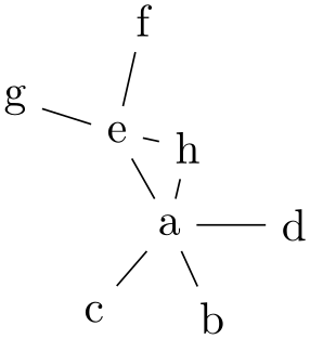
This key specifies that the straight line from the orient tail to the orient head should be at an angle of ⟨direction⟩ relative to the right-going \(x\)-axis. Which vertices are used as tail an head depends on where the orient option is encountered: When used with an edge, the tail is the edge’s tail and the head is the edge’s head. When used with a node, the tail or the head must be specified explicitly and the node is used as the node missing in the specification. When used with a graph as a whole, both the head and tail nodes must be specified explicitly. Note that the ⟨direction⟩ is independent of the actual to-path of an edge, which might define a bend or more complicated shapes. For instance, a ⟨angle⟩ of 45 requests that the end node is “up and right” relative to the start node.
You can also specify the standard direction texts north or south east and so forth as ⟨direction⟩ and also up, down, left, and right. Also, you can specify - for “right” and | for “down”.
Examples
-
/graph drawing/orient'=⟨direction⟩(default 0) 
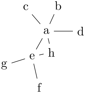
Same as orient, only the rest of the graph should be flipped relative to the connection line.
Example
-
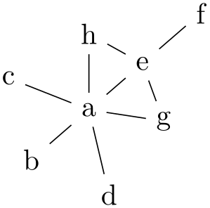
/graph drawing/orient tail=⟨string⟩ 
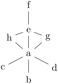
Specifies the tail vertex for the orientation of a graph. See orient for details.
Examples
                    \tikz \graph [spring layout] {

                      a [orient=|, orient tail=f] --
                    { b, c, d, e
                    -- {f, g, h} };

                      { h, g
                    } --
                    a;

                    };
                    \tikz \graph [spring layout] {

                      a [orient=down, orient tail=h] --
                    { b, c, d, e
                    -- {f, g, h} };

                      { h, g
                    } --
                    a;

                    };
-
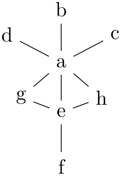
/graph drawing/orient head=⟨string⟩ 
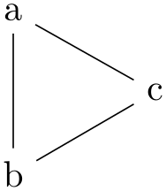
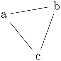
Specifies the head vertex for the orientation of a graph. See orient for details.
Examples
                    \tikz \graph [spring layout]

                    {

                      a [orient=|, orient head=f] --
                    { b, c, d, e
                    -- {f, g, h} };

                      { h, g
                    } --
                    a;

                    };
                    \tikz \graph [spring layout] { a
                    --
                    b
                    --
                    c
                    --
                    a };

                    \tikz \graph [spring layout, orient=10,

                                  orient tail=a, orient head=b] { a
                    --
                    b
                    --
                    c
                    --
                    a };
-
/graph drawing/horizontal=⟨string⟩ 
A shorthand for specifying orient tail, orient head and orient=0. The tail will be everything before the part “ to ” and the head will be everything following it.
Example

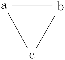
                    \tikz \graph [spring layout]                    { a
                    --
                    b
                    --
                    c
                    --
                    a };

                    \tikz \graph [spring layout, horizontal=a to b] { a
                    --
                    b
                    --
                    c
                    --
                    a };
-
/graph drawing/horizontal'=⟨string⟩ 
Like horizontal, but with a flip.
-
/graph drawing/vertical=⟨string⟩ 
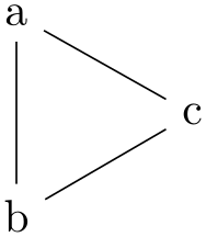
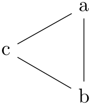
A shorthand for specifying orient tail, orient head and orient=-90.
Example
-
/graph drawing/vertical'=⟨string⟩ 
Like vertical, but with a flip.
-
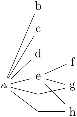
/graph drawing/grow=⟨direction⟩
This key specifies in which direction the neighbors of a node “should grow”. For some graph drawing algorithms, especially for those that layout trees, but also for those that produce layered layouts, there is a natural direction in which the “children” of a node should be placed. For instance, saying grow=down will cause the children of a node in a tree to be placed in a left-to-right line below the node (as always, you can replace the ⟨angle⟩ by direction texts). The children are requested to be placed in a counter-clockwise fashion, the grow' key will place them in a clockwise fashion. Note that when you say grow=down, it is not necessarily the case that any particular node is actually directly below the current node; the key just requests that the direction of growth is downward.
In principle, you can specify the direction of growth for each node individually, but do not count on graph drawing algorithms to honor these wishes.
When you give the grow=right key to the graph as a whole, it will be applied to all nodes. This happens to be exactly what you want:
Examples

                    \tikz \graph [layered layout, sibling distance=5mm]

                    {

                      a [grow=right] -- { b, c, d, e
                    -- {f, g, h} };

                      { h, g
                    } --
                    a;

                    };

                    \tikz \graph [layered layout, grow=right, sibling distance=5mm]

                    {

                      a
                    -- { b, c, d, e
                    -- {f, g, h} };

                      { h, g
                    } --
                    a;

                    };
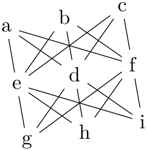
                    \tikz

                      \graph [layered layout, grow=-80]

                      {

                        {a,b,c} --[complete bipartite] {e,d,f}

                                --[complete bipartite] {g,h,i};

                      };
-
/graph drawing/grow'=⟨direction⟩
Same as grow, only with the children in clockwise order.
Example
                    \tikz \graph [layered layout, sibling distance=5mm]

                    {

                      a [grow'=right] -- { b, c, d, e
                    -- {f, g, h} };

                      { h, g
                    } --
                    a;

                    };
28.6 Fine-Tuning Positions of Nodes
-
/graph drawing/nudge=⟨canvas coordinate⟩ 
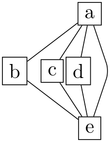
This option allows you to slightly “nudge” (move) nodes after they have been positioned by the given offset. The idea is that this nudging is done after the position of the node has been computed, so nudging has no influence on the actual graph drawing algorithms. This, in turn, means that you can use nudging to “correct” or “optimize” the positioning of nodes after the algorithm has computed something.
Example

-
/graph drawing/nudge up=⟨length⟩ 
A shorthand for nudging a node upwards.
Example

-
/graph drawing/nudge down=⟨length⟩ 
Like nudge up, but downwards.
-
/graph drawing/nudge left=⟨length⟩ 
Like nudge up, but left.
Example
                    \tikz \graph [edges=rounded corners, nodes=draw,

                                  layered layout, sibling distance=0] {

                      a
                    -- {b, c, d[nudge left=2mm]} --
                    e
                    --
                    a;

                    };
-
/graph drawing/nudge right=⟨length⟩ 
Like nudge left, but right.
-
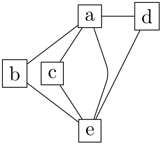
/graph drawing/regardless at=⟨canvas coordinate⟩ 
Using this option you can provide a position for a node to wish it will be forced after the graph algorithms have run. So, the node is positioned normally and the graph drawing algorithm does not know about the position specified using regardless at. However, afterwards, the node is placed there, regardless of what the algorithm has computed (all other nodes are unaffected).
Example
                    \tikz \graph [edges=rounded corners, nodes=draw,

                                  layered layout, sibling distance=0] {

                      a
                    -- {b,c,d[regardless at={(1,0)}]} --
                    e
                    --
                    a;

                    };
-
/graph drawing/nail at=⟨canvas coordinate⟩ 
This option combines desired at and regardless at. Thus, the algorithm is “told” about the desired position. If it fails to place the node at the desired position, it will be put there regardless. The name of the key is intended to remind one of a node being “nailed” to the canvas.
Example

28.7 Packing of Connected Components
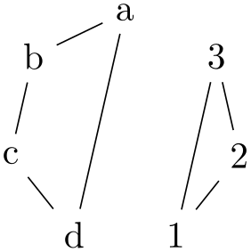
Graphs may be composed of subgraphs or components that are not connected to each other. In order to draw these nicely, most graph drawing algorithms split them into separate graphs, compute their layouts with the same graph drawing algorithm independently and, in a postprocessing step, arrange them next to each other. Note, however, that some graph drawing algorithms can also arrange the nodes of the graph in a uniform way even for unconnected components (the simple necklace layout is a case in point); for such algorithms you can choose whether they should be applied to each component individually or not (if not, the following options do not apply). To configure which is the case, use the componentwise key.
The default method for placing the different components works as follows:
-
1. For each component, a layout is determined and the component is oriented as described Section 28.5 on the orientation of graphs.
-
2. The components are sorted as prescribed by the component order key.
-
3. The first component is now placed (conceptually) at the origin. (The final position of this and all other components will be determined later, namely in the anchoring phase, but let us imagine that the first component lies at the origin at this point.)
-
4. The second component is now positioned relative to the first component. The “direction” in which the next component is placed relative to the first one is determined by the component direction key, so components can be placed from left to right or up to down or in any other direction (even something like \(30^\circ \)). However, both internally and in the following description, we assume that the components are placed from left to right; other directions are achieved by doing some (clever) rotating of the arrangement achieved in this way.
So, we now wish to place the second component to the right of the first component. The component is first shifted vertically according to some alignment strategy. For instance, it can be shifted so that the topmost node of the first component and the topmost node of the second component have the same vertical position. Alternatively, we might require that certain “alignment nodes” in both components have the same vertical position. There are several other strategies, which can be configured using the component align key.
One the vertical position has been fixed, the horizontal position is computed. Here, two different strategies are available: First, image rectangular bounding boxed to be drawn around both components. Then we shift the second component such that the right border of the bounding box of the first component touches the left border of the bounding box of the second component. Instead of having the bounding boxes “touch”, we can also have a padding of component sep between them. The second strategy is more involved and also known as a “skyline” strategy, where (roughly) the components are “moved together as near as possible so that nodes do not touch”.
-
5. After the second component has been placed, the third component is considered and positioned relative to the second one, and so on.
-
6. At the end, as hinted at earlier, the whole arrangement is rotate so that instead of “going right” the component go in the direction of component direction. Note, however, that this rotation applies only to the “shift” of the components; the components themselves are not rotated. Fortunately, this whole rotation process happens in the background and the result is normally exactly what you would expect.
In the following, we go over the different keys that can be used to configure the component packing.
-
/graph drawing/componentwise=⟨boolean⟩(default true) 
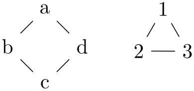
For algorithms that also support drawing unconnected graphs, use this key to enforce that the components of the graph are, nevertheless, laid out individually. For algorithms that do not support laying out unconnected graphs, this option has no effect; rather it works as if this option were always set.
Examples
,
28.7.1 Ordering the Components
The different connected components of the graph are collected in a list. The ordering of the nodes in this list can be configured using the following key.
-
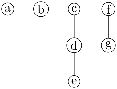
/graph drawing/component order=⟨string⟩(initially by first specified node) 
-
• by first specified node
The components are ordered “in the way they appear in the input specification of the graph”. More precisely, for each component consider the node that is first encountered in the description of the graph. Order the components in the same way as these nodes appear in the graph description.
-
• increasing node number
The components are ordered by increasing number of nodes. For components with the same number of nodes, the first node in each component is considered and they are ordered according to the sequence in which these nodes appear in the input.
-
• decreasing node number As above, but in decreasing order.
Selects a “strategy” for ordering the components. By default, they are ordered in the way they appear in the input. The following values are permissible for ⟨strategy⟩
Examples

-
/graph drawing/small components first=⟨string⟩ 
A shorthand for component order=increasing node number.

28.7.2 Arranging Components in a Certain Direction
-
/graph drawing/component direction=⟨direction⟩(initially 0) 
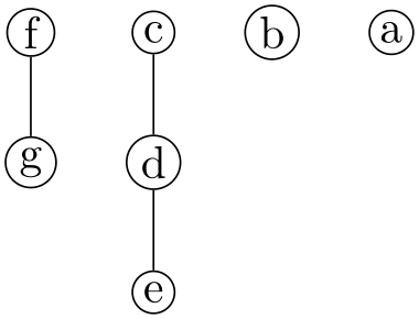
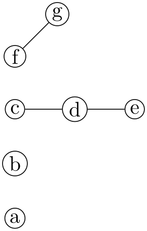
The ⟨angle⟩ is used to determine the relative position of each component relative to the previous one. The direction need not be a multiple of 90. As usual, you can use texts like up or right instead of a number. As the examples show, the direction only has an influence on the relative positions of the components, not on the direction of growth inside the components. In particular, the components are not rotated by this option in any way. You can use the grow option or orient options to orient individual components.
Examples
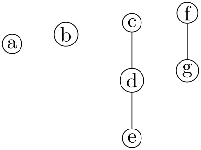
                    \tikz \graph [tree layout, nodes={inner sep=1pt,draw,circle},

                                  component direction=10]

                      { a, b, c
                    --
                    d
                    --
                    e, f
                    --
                    g };
28.7.3 Aligning Components
When components are placed next to each from left to right, it is not immediately clear how the components should be aligned vertically. What happens is that in each component a horizontal line is determined and then all components are shifted vertically so that the lines are aligned. There are different strategies for choosing these “lines”, see the description of the options described later on. When the component direction option is used to change the direction in which components are placed, it certainly make no longer sense to talk about “horizontal” and “vertical” lines. Instead, what actually happens is that the alignment does not consider “horizontal” lines, but lines that go in the direction specified by component direction and aligns them by moving components along a line that is perpendicular to the line. For these reasons, let us call the line in the component direction the alignment line and a line that is perpendicular to it the shift line.
The first way of specifying through which point of a component the alignment line should get is to use the option align here. In many cases, however, you will not wish to specify an alignment node manually in each component. Instead, you will use the component align key to specify a strategy that should be used to automatically determine such a node.
Using a combination of component direction and component align, numerous different packing strategies can be configured. However, since names like counterclockwise are a bit hard to remember and to apply in practice, a number of easier-to-remember keys are predefined that combine an alignment and a direction.
-
/graph drawing/align here=⟨boolean⟩(default true) 
When this option is given to a node, this alignment line will go through the origin of this node. If this option is passed to more than one node of a component, the node encountered first in the component is used.
Example

                    \tikz \graph [binary tree layout, nodes={draw}]

                      { a, b
                    --
                    c[align here], d
                    --
                    e[second, align here] --
                    f };
-
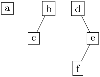
/graph drawing/component align=⟨string⟩(initially first node) 
-
• first node
In each component, the alignment line goes through the center of the first node of the component encountered during specification of the component.
-
• center
The nodes of the component are projected onto the shift line. The alignment line is now chosen so that it is exactly in the middle between the maximum and minimum value that the projected nodes have on the shift line.
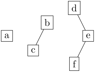
                        \usetikzlibrary {graphs,graphdrawing} \usegdlibrary {trees}

                        \tikz \graph [binary tree layout, nodes={draw},

                                      component align=center]

                          { a, b
                        --
                        c, d
                        --
                        e[second] --
                        f };

                        \usetikzlibrary {graphs,graphdrawing} \usegdlibrary {trees}

                        \tikz \graph [binary tree layout, nodes={draw},

                                      component direction=90,

                                      component align=center]

                          { a, b
                        --
                        c, d
                        --
                        e[second] --
                        f };
-
• counterclockwise
As for center, we project the nodes of the component onto the shift line. The alignment line is now chosen so that it goes through the center of the node whose center has the highest projected value.
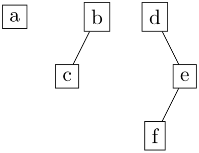
                        \usetikzlibrary {graphs,graphdrawing} \usegdlibrary {trees}

                        \tikz \graph [binary tree layout, nodes={draw},

                                      component align=counterclockwise]

                          { a, b
                        --
                        c, d
                        --
                        e[second] --
                        f };

                        \usetikzlibrary {graphs,graphdrawing} \usegdlibrary {trees}

                        \tikz \graph [binary tree layout, nodes={draw},

                                      component direction=90,

                                      component align=counterclockwise]

                         { a, b
                        --
                        c, d
                        --
                        e[second] --
                        f };
The name counterclockwise is intended to indicate that the align line goes through the node that comes last if we go from the alignment direction in a counter-clockwise direction.
-
• clockwise
Works like counterclockwise, only in the other direction:
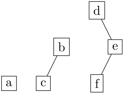

                        \usetikzlibrary {graphs,graphdrawing} \usegdlibrary {trees}

                        \tikz \graph [binary tree layout, nodes={draw},

                                      component direction=90,

                                      component align=clockwise]

                          { a, b
                        --
                        c, d
                        --
                        e[second] --
                        f };
-
• counterclockwise bounding box
This method is quite similar to counterclockwise, only the alignment line does not go through the center of the node with a maximum projected value on the shift line, but through the maximum value of the projected bounding boxes. For a left-to-right packing, this means that the components are aligned so that the bounding boxes of the components are aligned at the top.
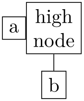
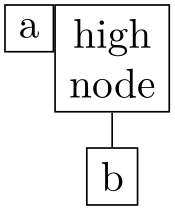
                        \usetikzlibrary {graphs,graphdrawing} \usegdlibrary {trees}

                        \tikz \graph [tree layout, nodes={draw, align=center},

                                      component sep=0pt,

                                      component align=counterclockwise]

                          { a, "high\\node"
                        --
                        b};\quad

                        \tikz \graph [tree layout, nodes={draw, align=center},

                                      component sep=0pt,

                                      component align=counterclockwise bounding box]

                          { a, "high\\node"
                        --
                        b};
-
• clockwise bounding box
Works like counterclockwise bounding box.
Specifies a “strategy” for the alignment of components. The following values are permissible:
-
/graph drawing/components go right top aligned=⟨string⟩ 
Shorthand for component direction=right and component align=counterclockwise. This means that, as the name suggest, the components will be placed left-to-right and they are aligned such that their top nodes are in a line.
Example

                    \tikz \graph [tree layout, nodes={draw, align=center},

                                  components go right top aligned]

                      { a, "high\\node"
                    --
                    b};
-
/graph drawing/components go right absolute top aligned=⟨string⟩ 
Like components go right top aligned, but with component align set to counterclockwise bounding box. This means that the components will be aligned with their bounding boxed being top-aligned.
Example
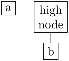
                    \tikz \graph [tree layout, nodes={draw, align=center},

                                  components go right absolute top aligned]

                      { a, "high\\node"
                    --
                    b};
-
/graph drawing/components go right bottom aligned=⟨string⟩ 
See the other components go ... keys.
-
/graph drawing/components go right absolute bottom aligned=⟨string⟩ 
See the other components go ... keys.
-
/graph drawing/components go right center aligned=⟨string⟩ 
See the other components go ... keys.
-
/graph drawing/components go right=⟨string⟩ 
Shorthand for component direction=right and component align=first node.
-
/graph drawing/components go left top aligned=⟨string⟩ 
See the other components go ... keys.
Example
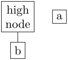
                    \tikz \graph [tree layout, nodes={draw, align=center},

                                  components go left top aligned]

                      { a, "high\\node"
                    --
                    b};
-
/graph drawing/components go left absolute top aligned=⟨string⟩ 
See the other components go ... keys.
-
/graph drawing/components go left bottom aligned=⟨string⟩ 
See the other components go ... keys.
-
/graph drawing/components go left absolute bottom aligned=⟨string⟩ 
See the other components go ... keys.
-
/graph drawing/components go left center aligned=⟨string⟩ 
See the other components go ... keys.
-
/graph drawing/components go left=⟨string⟩ 
See the other components go ... keys.
-
/graph drawing/components go down right aligned=⟨string⟩ 
See the other components go ... keys.
Examples
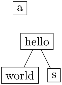
                    \tikz \graph [tree layout, nodes={draw, align=center},

                                  components go down left aligned]

                      { a, hello
                    -- {world,s} };
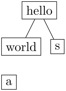
                    \tikz \graph [tree layout, nodes={draw, align=center},

                                  components go up absolute left aligned]

                      { a, hello
                    -- {world,s}};
-
/graph drawing/components go down absolute right aligned=⟨string⟩ 
See the other components go ... keys.
-
/graph drawing/components go down left aligned=⟨string⟩ 
See the other components go ... keys.
-
/graph drawing/components go down absolute left aligned=⟨string⟩ 
See the other components go ... keys.
-
/graph drawing/components go down center aligned=⟨string⟩ 
See the other components go ... keys.
-
/graph drawing/components go down=⟨string⟩ 
See the other components go ... keys.
-
/graph drawing/components go up right aligned=⟨string⟩ 
See the other components go ... keys.
-
/graph drawing/components go up absolute right aligned=⟨string⟩ 
See the other components go ... keys.
-
/graph drawing/components go up left aligned=⟨string⟩ 
See the other components go ... keys.
-
/graph drawing/components go up absolute left aligned=⟨string⟩ 
See the other components go ... keys.
-
/graph drawing/components go up center aligned=⟨string⟩ 
See the other components go ... keys.
-
/graph drawing/components go up=⟨string⟩ 
See the other components go ... keys.
28.7.4 The Distance Between Components
Once the components of a graph have been oriented, sorted, aligned, and a direction has been chosen, it remains to determine the distance between adjacent components. Two methods are available for computing this distance, as specified by the following option:
-
/graph drawing/component packing=⟨string⟩(initially skyline) 
-
• rectangular
Imagine a bounding box to be drawn around both components. They are then shifted such that the padding (separating distance) between the two boxes is the current value of component sep.

                        \usetikzlibrary {graphs,graphdrawing} \usegdlibrary {trees}

                            \tikz \graph [tree layout, nodes={draw}, component sep=0pt,

                                          component packing=rectangular]

                              { a
                        --
                        long
                        text, longer
                        text
                        --
                        b};
-
• skyline
The “skyline method” is used to compute the distance. It works as follows: For simplicity, assume that the component direction is right (other case work similarly, only everything is rotated). Imaging the second component to be placed far right beyond the first component. Now start moving the second component back to the left until one of the nodes of the second component touches a node of the first component, and stop. Again, the padding component sep can be used to avoid the nodes actually touching each other.

                        \usetikzlibrary {graphs,graphdrawing} \usegdlibrary {trees}

                            \tikz \graph [tree layout, nodes={draw}, component sep=0pt,

                                          level distance=1.5cm,

                                          component packing=skyline]

                              { a
                        --
                        long
                        text, longer
                        text
                        --
                        b};
In order to avoid nodes of the second component “passing through a hole in the first component”, the actual algorithm is a bit more complicated: For both components, a “skyline” is computed. For the first component, consider an arbitrary horizontal line. If there are one or more nodes on this line, the rightmost point on any of the bounding boxes of these nodes will be the point on the skyline of the first component for this line. Similarly, for the second component, for each horizontal level the skyline is given by the leftmost point on any of the bounding boxes intersecting the line.
Now, the interesting case are horizontal lines that do not intersect any of the nodes of the first and/or second component. Such lines represent “holes” in the skyline. For them, the following rule is used: Move the horizontal line upward and downward as little as possible until a height is reached where there is a skyline defined. Then the skyline position on the original horizontal line is the skyline position at the reached line, minus (or, for the second component, plus) the distance by which the line was moved. This means that the holes are “filled up by slanted roofs”.

                        \usetikzlibrary {graphs,graphdrawing} \usegdlibrary {trees}

                            \begin{tikzpicture}

                              \graph [tree layout, nodes={draw}, component sep=0pt,

                                      component packing=skyline]

                              { a
                        --
                        long
                        text, longer
                        text
                        --
                        b};

                              \draw[red] (long text.north east) --
                        ++(north west:1cm);

                            \end{tikzpicture}
Given two components, their distance is computed as follows in dependence of ⟨method⟩:
28.8 Anchoring Edges
When a graph has been laid out completely, the edges between the nodes must be drawn. Conceptually, an edge is “between two nodes”, but when we actually draw the node, we do not really want the edge’s path to start “in the middle” of the node; rather, we want it to start “on the border” and also end there.
Normally, computing such border positions for nodes is something we would leave to the so-called display layer (which is typically TikZ and TikZ is reasonably good at computing border positions). However, different display layers may behave differently here and even TikZ fails when the node shapes are very involved and the paths also.
For these reasons, computing the anchor positions where edges start and end is done inside the graph drawing system. As a user, you specify a tail anchor and a head anchor, which are points inside the tail and head nodes, respectively. The edge path will then start and end at these points, however, they will usually be shortened so that they actually start and end on the intersection of the edge’s path with the nodes’ paths.
-
/graph drawing/tail anchor=⟨string⟩ 
Specifies where in the tail vertex the edge should start. This is either a string or a number, interpreted as an angle (with 90 meaning “up”). If it is a string, when the start of the edge is computed, we try to look up the anchor in the tail vertex’s table of anchors (some anchors get installed in this table by the display system). If it is not found, we test whether it is one of the special “direction anchors” like north or south east. If so, we convert them into points on the border of the node that lie in the direction of a line starting at the center to a point on the bounding box of the node in the designated direction. Finally, if the anchor is a number, we use a point on the border of the node that is on a line from the center in the specified direction.
If the anchor is set to the empty string (which is the default), the anchor is interpreted as the center anchor inside the graph drawing system. However, a display system may choose to make a difference between the center anchor and an empty anchor (TikZ does: for options like bend left if the anchor is empty, the bend line starts at the border of the node, while for the anchor set explicitly to center it starts at the center).
Note that graph drawing algorithms need not take the setting of this option into consideration. However, the final rendering of the edge will always take it into consideration (only, the setting may not be very sensible if the algorithm ignored it).
-
/graph drawing/head anchor=⟨string⟩ 
See tail anchor
-
/graph drawing/tail cut=⟨boolean⟩(default true, initially true) 
Decides whether the tail of an edge is “cut”, meaning that the edge’s path will be shortened at the beginning so that it starts only of the node’s border rather than at the exact position of the tail anchor, which may be inside the node.
-
/graph drawing/head cut=⟨boolean⟩(default true, initially true) 
See tail cut.
-
/graph drawing/cut policy=⟨string⟩(initially as edge requests) 
-
• as edge requests Whether or not an edge entering or leaving the node is cut depends on the setting of the edge’s tail cut and head cut options. This is the default.
-
• all All edges entering or leaving the node are cut, regardless of the edges’ cut values.
-
• none No edge entering or leaving the node is cut, regardless of the edges’ cut values.
The policy for cutting edges entering or leaving a node. This option is important for nodes only. It can have three possible values:
-
/graph drawing/allow inside edges=⟨boolean⟩(default true, initially true) 
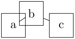
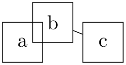
Decides whether an edge between overlapping nodes should be drawn. If two vertices overlap, it may happen that when you draw an edge between them, this edges would be completely inside the two vertices. In this case, one could either not draw them or one could draw a sort of “inside edge”.
Examples
28.9 Hyperedges
-
/graph drawing/hyper(style) 
A hyperedge of a graph does not connect just two nodes, but is any subset of the node set (although a normal edge is also a hyperedge that happens to contain just two nodes). Internally, a collection of kind hyper is created. Currently, there is no default renderer for hyper edges.
28.10 Using Several Different Layouts to Draw a Single Graph
Inside each graph drawing scope, a main algorithm is used to perform the graph drawing. However, parts of the graph may be drawn using different algorithms: For instance, a graph might consist of several, say, cliques that are arranged in a tree-like fashion. In this case, it might be useful to layout each clique using a circular layout, but then lay out all laid out cliques using a tree drawing algorithm.
In order to lay out a graph using multiple algorithms, we need two things: First, we must be able to specify which algorithms should be used where and, second, we must be able to resolve conflicts that may result from different algorithms “having different ideas” concerning where nodes should be placed.
28.10.1 Sublayouts
Specifying different layouts for a graph is easy: Inside a graph drawing scope, simply open scopes, in which you use an option like tree layout for the nodes mentioned in this scope. Inside these scopes, you can open even subscopes for sublayouts, and so on. Furthermore, the graphs library has special support for sublayouts.
Let us start with the “plain” syntax for opening sublayouts: You pass a key for creating layouts to a scope:

                \usetikzlibrary {graphdrawing} \usegdlibrary {force,trees}

                \tikz [spring layout] {

                  \begin{scope}[tree layout]

                    \node (a) {a};

                    \node (b) {b};

                    \node (c) {c};

                    \draw (a) edge
                (b) edge
                (c);

                  \end{scope}


                  \begin{scope}[tree layout]

                    \node (1) {1};

                    \node (2) {2};

                    \draw (1) edge
                (2);

                  \end{scope}


                  \draw (a) edge
                (1);

                }
Let us see, what is going on here. The main layout (spring layout) contains two sublayouts (the two tree layouts). Both of them are laid out independently (more on the details in a moment). Then, from the main layout’s point of view, the sublayouts behave like “large nodes” and, thus, the edge between a and 1 is actually the only edge that is used by the spring layout – resulting in a simple layout consisting of one big node at the top and a big node at the bottom.
The graphs library has a special support for sublayouts: The syntax is as follows: wherever a normal node would go, you can write
// [⟨layout options⟩] {⟨sublayout⟩}
Following the double slash, you may provide ⟨layout options⟩ in square brackets. However, you must provide a sublayout in braces. The contents of ⟨sublayout⟩ will be parsed using the usual graph syntax, but will form a sublayout.
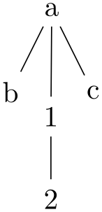
                \usetikzlibrary {graphs,graphdrawing} \usegdlibrary {force,trees}

                \tikz \graph [spring layout] {

                  // [tree layout] { a
                -- {b, c} };

                  // [tree layout] { 1
                --
                2 };

                  a
                --
                1;

                };
In the above example, there is no node before the double slash, which means that the two sublayouts will be part of the main graph, but will not be indicated otherwise.

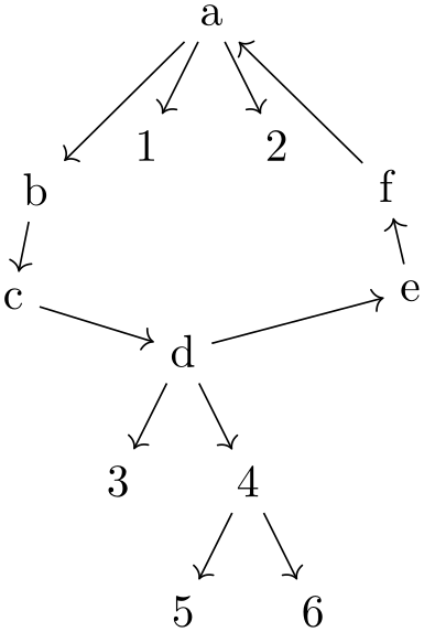
                \usetikzlibrary {graphs,graphdrawing} \usegdlibrary {circular,trees}

                \tikz \graph [simple necklace layout] {

                 // [simple necklace layout] { a
                ->
                b
                ->
                c
                ->
                d
                ->
                e
                ->
                f
                ->
                a };


                 // [tree layout] { % first tentacle

                   a
                -> {1, 2};

                 };


                 // [tree layout] {% second tentacle

                   d
                -> {3, 4
                -> {5, 6}}

                 };

                };
In the above example, the first sublayout is the one for the nodes with letter names. These nodes are arranged using a simple necklace layout as the sublayout inherits this option from the main layout. The two small trees (a -> {1, 2} and the tree starting at the d node) are also sublayouts, triggered by the tree layout option. They are also arranged. Then, all of the layouts are merged (as described later). The result is actually a single node, so the main layout does nothing here.
Compare the above to the following code:
                \usetikzlibrary {graphs,graphdrawing} \usegdlibrary {circular,trees}

                \tikz \graph [simple necklace layout] {

                  // [tree layout] { % first ``giant node''

                    a
                -> {1, 2};

                  };


                  a
                ->
                b
                ->
                c
                ->
                d;


                  // [tree layout] {% second ``giant node''

                    d
                -> {3, 4
                -> {5, 6}}

                  },


                  d
                ->
                e
                ->
                f
                ->
                a;

                };
Here, only the two trees are laid out first. They are then contracted into “giant nodes” and these are then part of the set of nodes that are arranged by the simple necklace layout. For details of how this contracting works, see below.
28.10.2 Subgraph Nodes
A subgraph node is a special kind of node that “surrounds” the vertices of a subgraph. The special property of a subgraph node opposed to a normal node is that it is created only after the subgraph has been laid out. However, the difference to a collection like hyper is that the node is available immediately as a normal node in the sense that you can connect edges to it.
The syntax used to declare a subgraph node in a graph specification is as follows:
"⟨node name⟩"/"⟨text⟩" [⟨node options⟩] // [⟨layout options⟩] {⟨subgraph⟩}
The idea ist that a subgraph node is declared like a normal node specification, but is followed by a double slash and a subgraph:
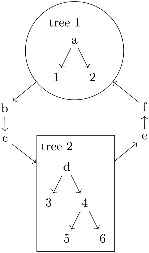
Note how the two subgraph nodes tree 1 and tree 2 surround the two smaller trees. In the example, both had trees as contents and these trees were rendered using a sublayout. However, a subgraph layout does not need to have its own layout: If you do not provide a layout name after the double slash, the subgraph node will simply surround all nodes that were placed by the main layout wherever they were placed:
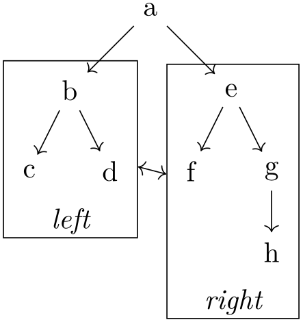
Every time a subgraph node is created, the following style is execute:
-
/tikz/every subgraph node(no value) 
Set a subgraph node style.
-
/tikz/subgraph nodes=⟨style⟩(no default) 
Sets the every subgraph node style to ⟨style⟩.

-
/tikz/subgraph text none(no value) 
When this option is used, the text of a subgraph node is not shown. Adding a slash after the node name achieves roughly the same effect, but this option is useful in situations when subgraph nodes generally should not have any text inside them.

-
/tikz/subgraph text top=⟨text alignment options⟩ (default text ragged right) 
Specifies that the text of a subgraph node should be placed at the top of the subgraph node: Still inside the node, but above all nodes inside the subgraph node.

You can pass any of the ⟨text alignment options⟩ understood by TikZ, such as text centered:

To place a label outside the subgraph node, use a label, typically defined using the quotes library:

-
/tikz/subgraph text bottom=⟨text alignment options⟩ (default ragged right) 
Works like subgraph text top, only the text placed at the bottom.
Note that there are no keys subgraph text left or ... right, for somewhat technical reasons.
-
/tikz/subgraph text sep=⟨dimension⟩ (no default, initially .1em) 
Some space added between the inner nodes of a subgraph node and the text labels.
28.10.3 Overlapping Sublayouts
Nodes and edges can be part of several layouts. This will inevitably lead to conflicts because algorithm will disagree on where a node should be placed on the canvas. For this reason, there are some rules governing how such conflicts are resolved: Given a layout, starting with the main layout, the graph drawing system does the following:
-
1. We start by first processing the (direct) sublayouts of the current layout (recursively). Sublayouts may overlap (they may share one or more nodes), but we run the specified layout algorithm for each sublayout independently on a “fresh copy” of all the nodes making up the sublayout. In particular, different, conflicting positions may be computed for nodes when they are present in several sublayouts.
-
2. Once all nodes in the sublayouts have been laid out in this way, we join overlapping elements. The idea is that if two layouts share exactly one vertex, we can shift them around so that his vertex is at the same position in both layouts. In more detail, the following happens:
We build a (conceptual) graph whose nodes are the sublayouts and in which there is an edge between two nodes if the sublayouts represented by these elements have a node in common. Inside the resulting graph, we treat each connected component separately. Each component has the property that the sublayouts represented by the nodes in the component overlap by at least one node. We now join them as follows: We start with the first sublayout in the component (“first” with respect to the order in which they appear in the input graph) and “mark” this sublayout. We loop the following instructions as long as possible: Search for the first sublayout (again, with respect to the order in which they appear in the input) that is connect by an edge to a marked sublayout. The sublayout will now have at least one node in common with the marked sublayouts (possibly, even more). We consider the first such node (again, first respect to the input ordering) and shift the whole sublayout is such a way that this particular node is at the position is has in the marked sublayouts. Note that after the shift, other nodes that are also present in the marked sublayouts may lie at a different position in the current sublayout. In this case, the position in the marked sublayouts “wins”. We then mark the sublayout.
-
3. When the above algorithm has run, we will have computed positions for all nodes in all sublayouts of each of the components. For each component, we contract all nodes of the component to a single node. This new node will be “large” in the sense that its convex hull is the convex hull of all the nodes in the component. All nodes that used to be part of the component are removed and the new large node is added (with arcs adjusted appropriately).
-
4. We now run the layout’s algorithm on the resulting nodes (the remaining original nodes and the contracted nodes).
-
5. In a last step, once the graph has been laid out, we expand the nodes that were previously contracted. For this, the nodes that were deleted earlier get reinserted, but shifted by whatever amount the contraction node got shifted.
28.11 Miscellaneous Options
-
/graph drawing/nodes behind edges=⟨boolean⟩(default true) 
Specifies, that nodes should be drawn behind the edges Once a graph drawing algorithm has determined positions for the nodes, they are drawn before the edges are drawn; after all, it is hard to draw an edge between nodes when their positions are not yet known. However, we typically want the nodes to be rendered after or rather on top of the edges. For this reason, the default behavior is that the nodes at their final positions are collected in a box that is inserted into the output stream only after the edges have been drawn – which has the effect that the nodes will be placed “on top” of the edges.
This behavior can be changed using this option. When the key is invoked, nodes are placed behind the edges.
Example
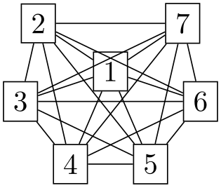
                    \tikz \graph [simple necklace layout, nodes={draw,fill=white},

                                  nodes behind edges]

                      { subgraph
                    K_n [n=7], 1
                    [regardless at={(0,-1)}] };
-
/graph drawing/edges behind nodes=⟨string⟩ 
This is the default placement of edges: Behind the nodes.
Example

                    \tikz \graph [simple necklace layout, nodes={draw,fill=white},

                                  edges behind nodes]

                      { subgraph
                    K_n [n=7], 1
                    [regardless at={(0,-1)}] };
-
/graph drawing/random seed=⟨number⟩(initially 42) 
To ensure that the same is always shown in the same way when the same algorithm is applied, the random is seed is reset on each call of the graph drawing engine. To (possibly) get different results on different runs, change this value.
-
/graph drawing/variation=⟨number⟩ 
An alias for random seed.
-
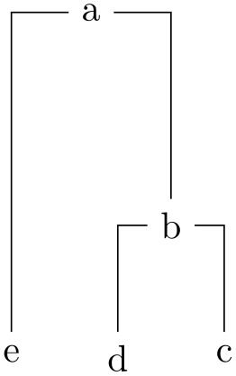
/graph drawing/weight=⟨number⟩(initially 1) 
Sets the “weight” of an edge or a node. For many algorithms, this number tells the algorithm how “important” the edge or node is. For instance, in a layered layout, an edge with a large weight will be as short as possible.
Examples
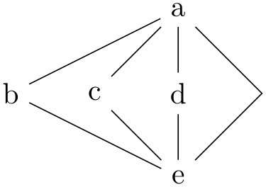
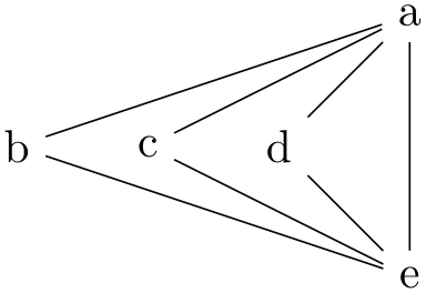
-
/graph drawing/length=⟨length⟩(initially 1)
Sets the “length” of an edge. Algorithms may take this value into account when drawing a graph.
Example
-
/graph drawing/radius=⟨number⟩(initially 0)
The radius of a circular object used in graph drawing.
-
/graph drawing/no layout=⟨string⟩ 
This layout does nothing.